Autonomous Cave Surveying with an Aerial Robot

TRO · 2022

King-Sun Fu Memorial Best Paper Award (Honorable Mention)

Caves are surveyed by hand using 2D instruments in hazardous conditions since the 19th century. How do we explore caves in 3D using aerial robots?

Wennie Tabib Kshitij Goel John Yao Curtis Boirum Nathan Michael

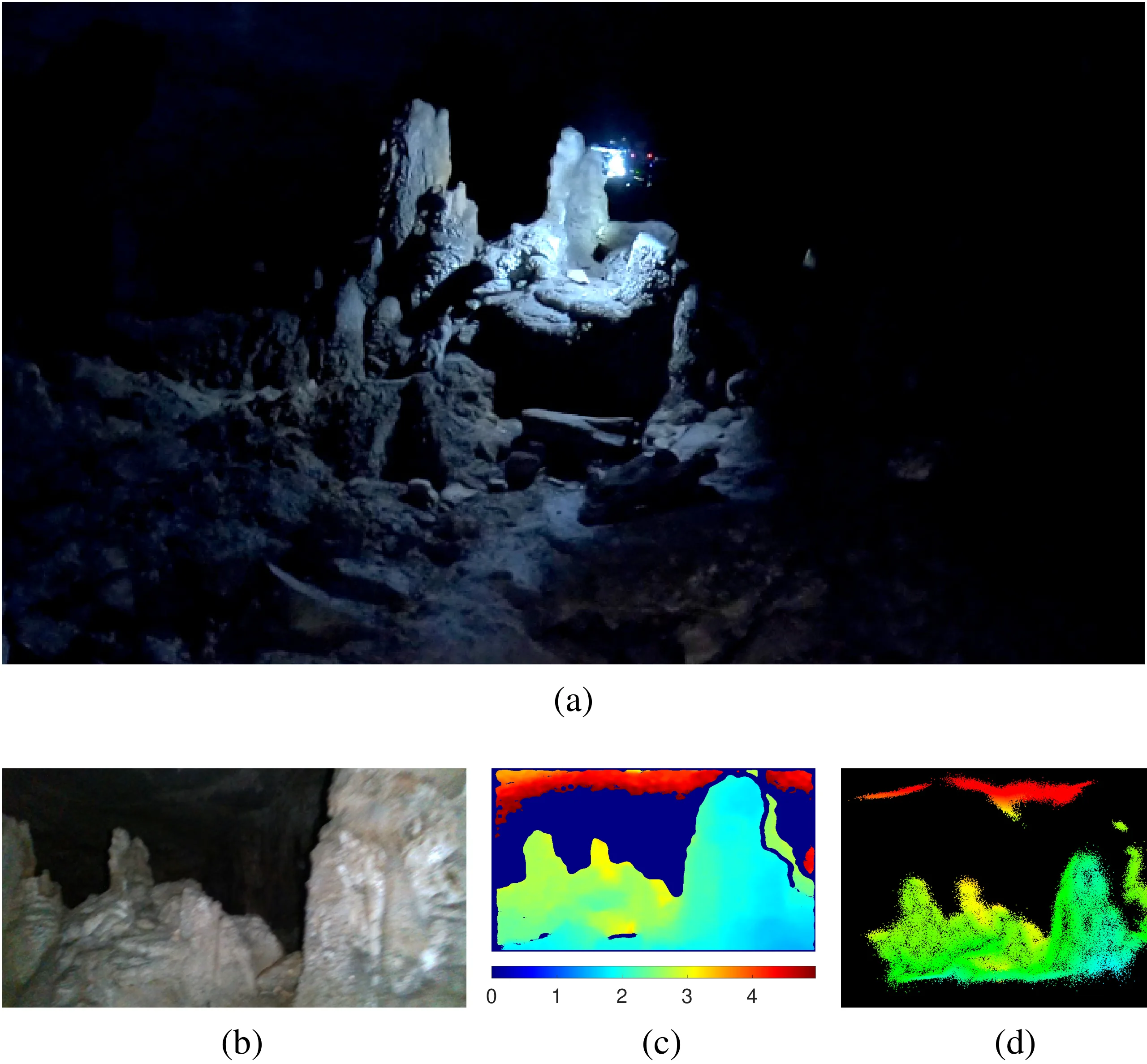
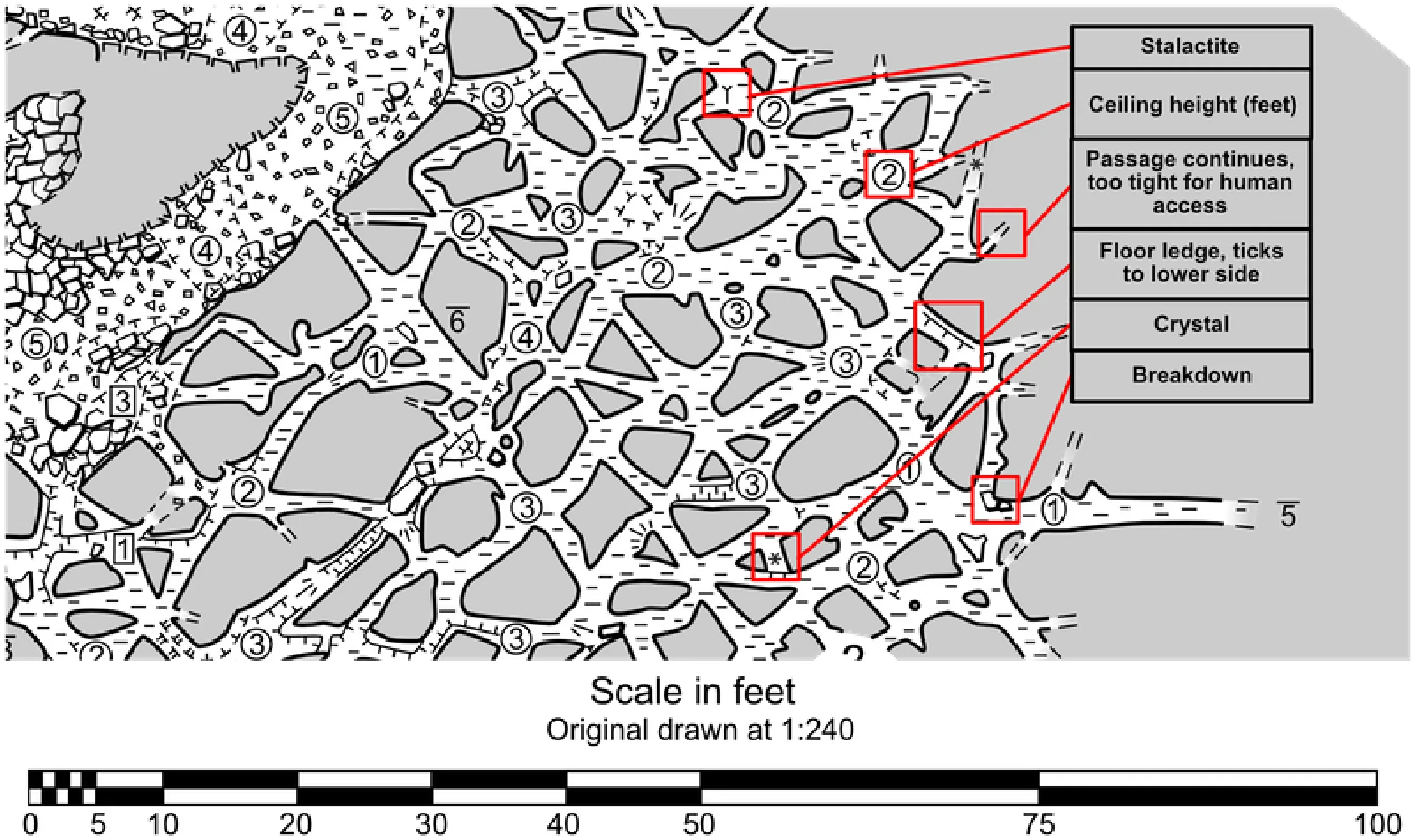
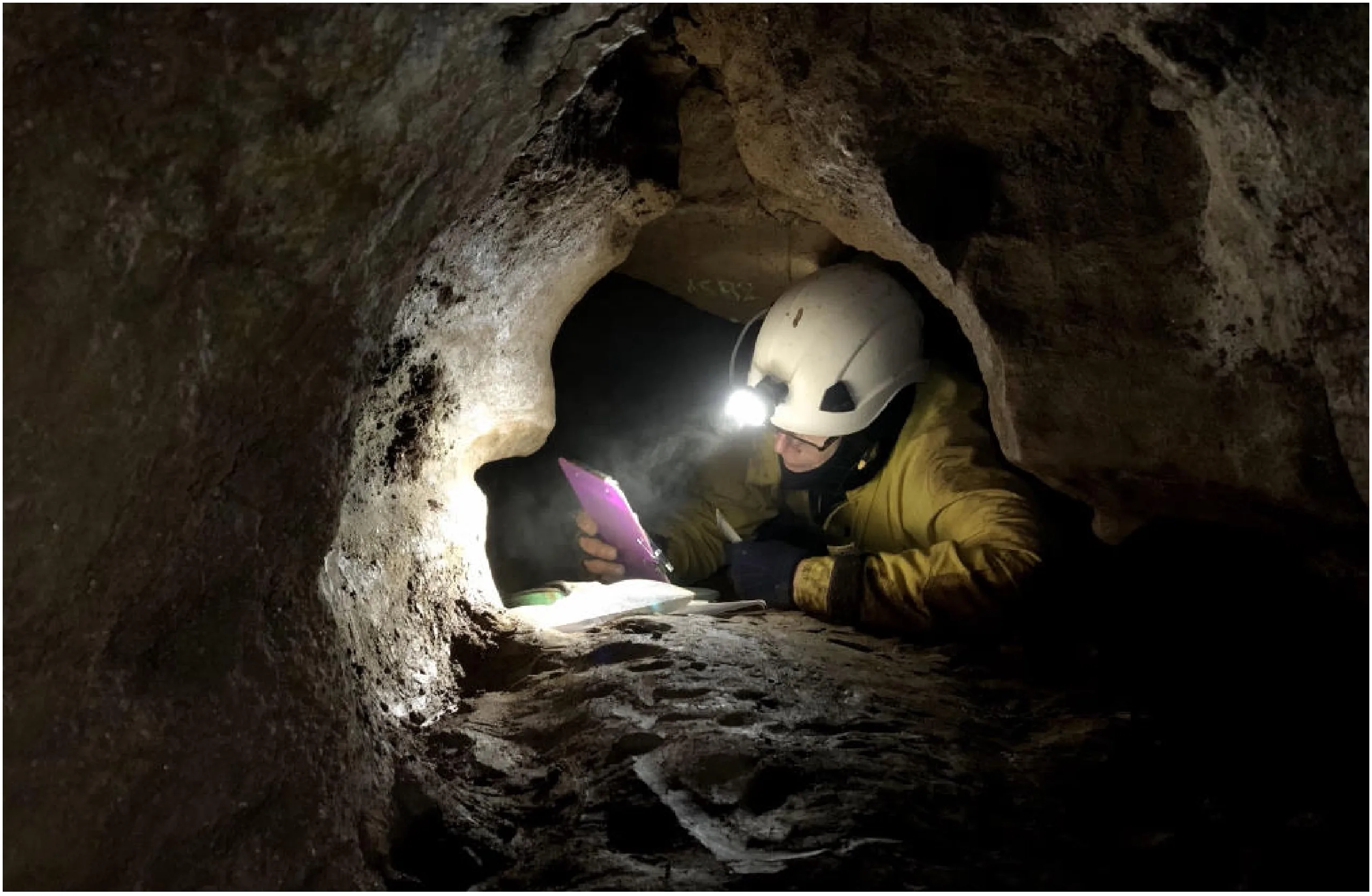
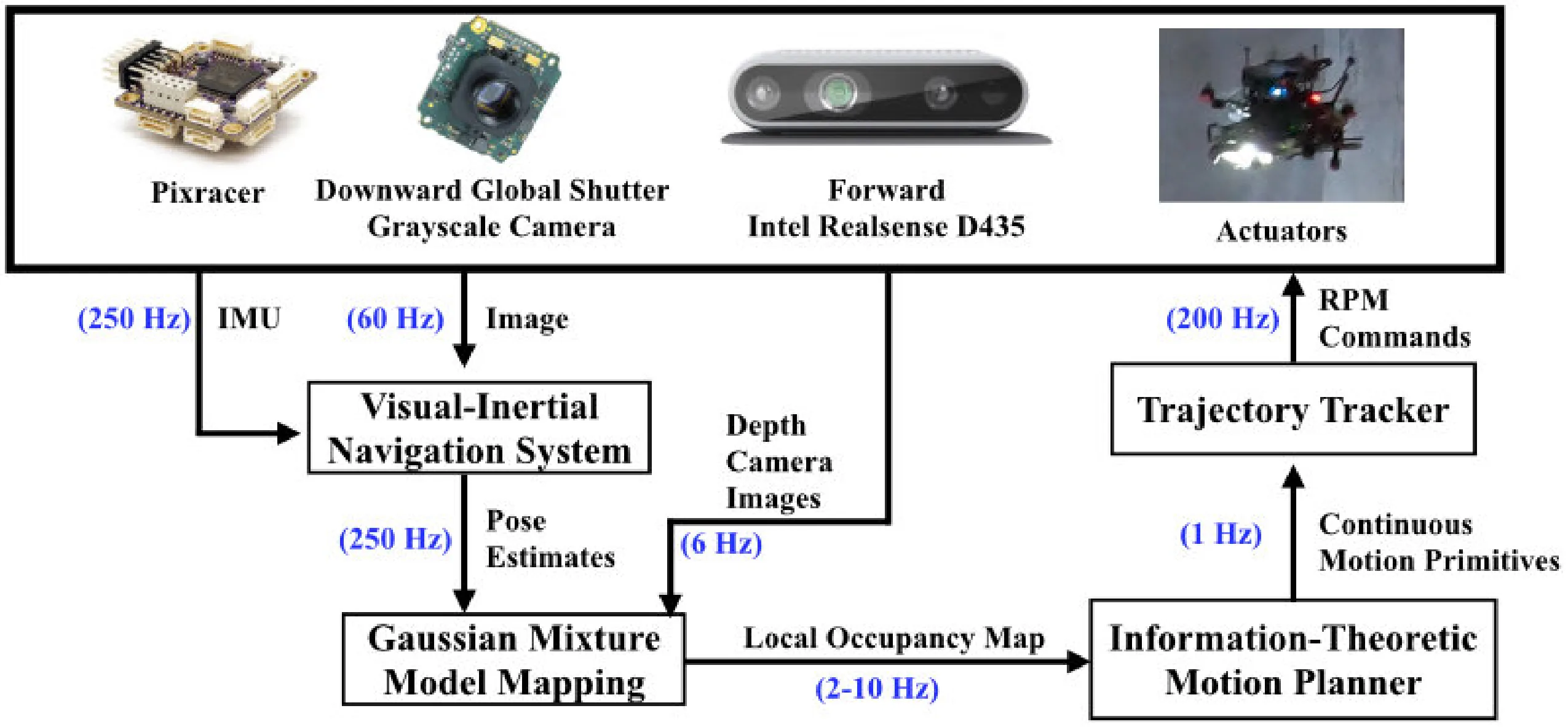
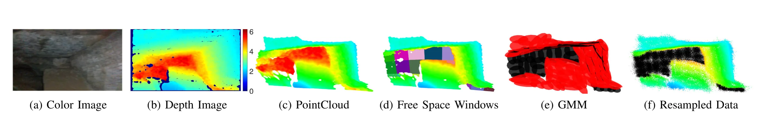
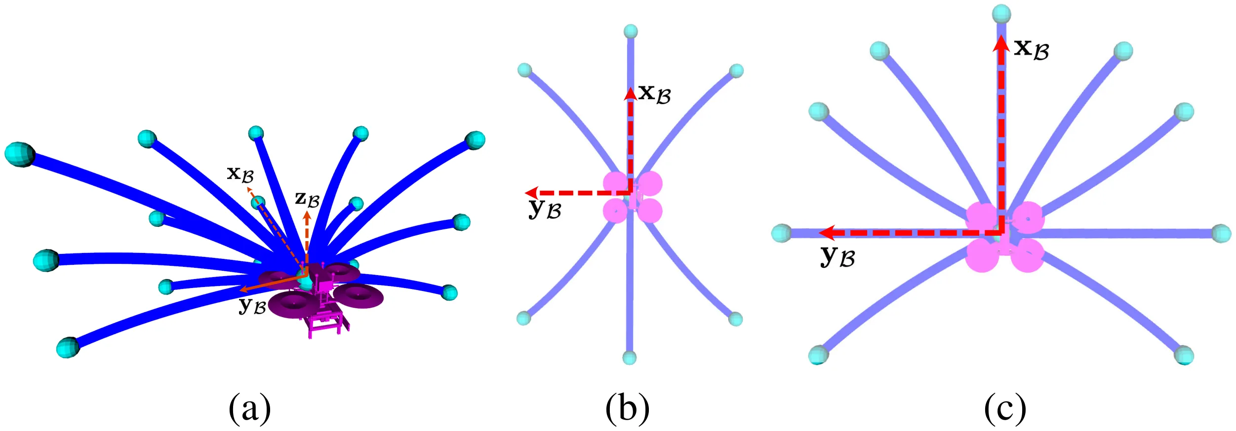
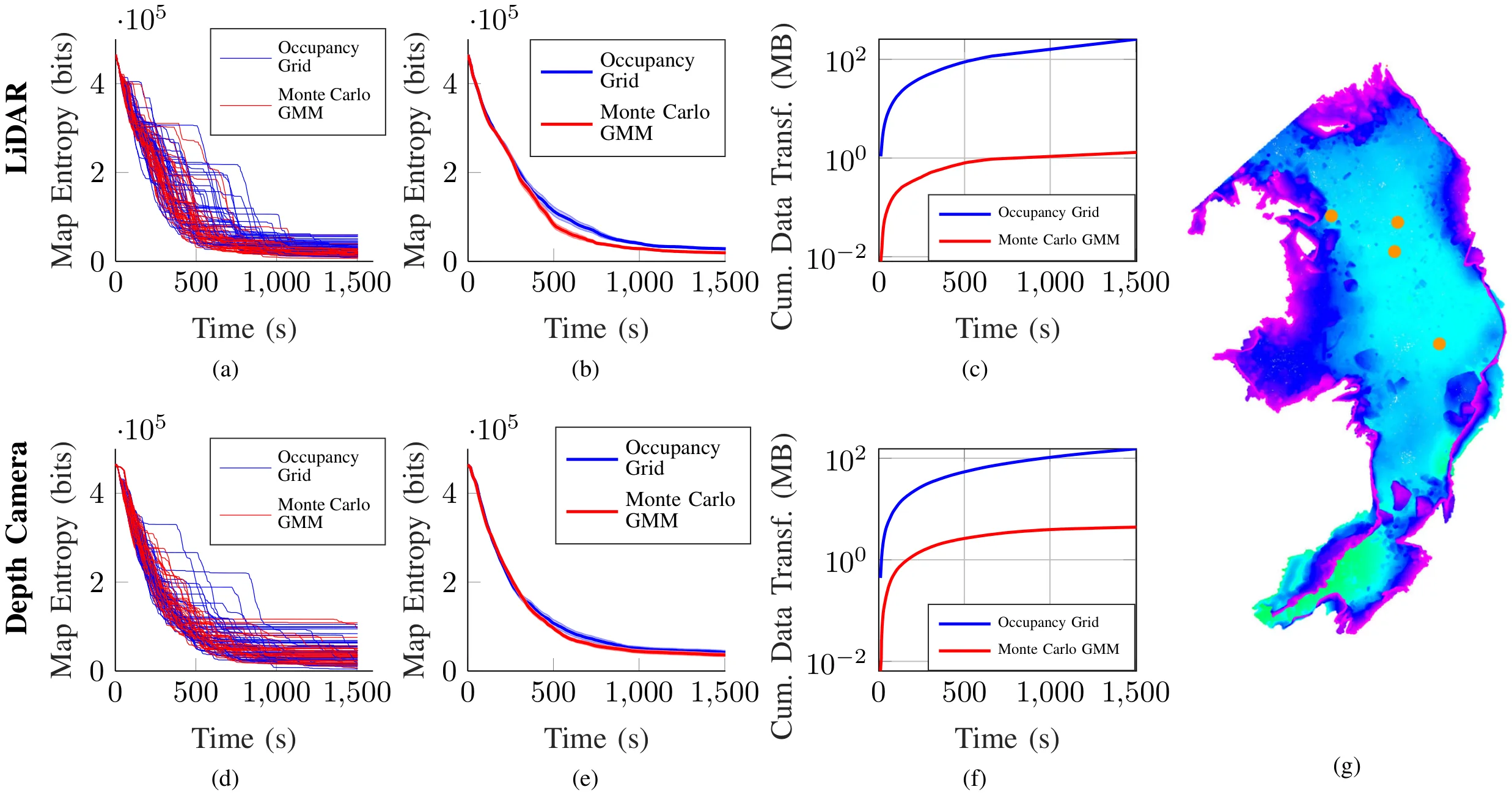
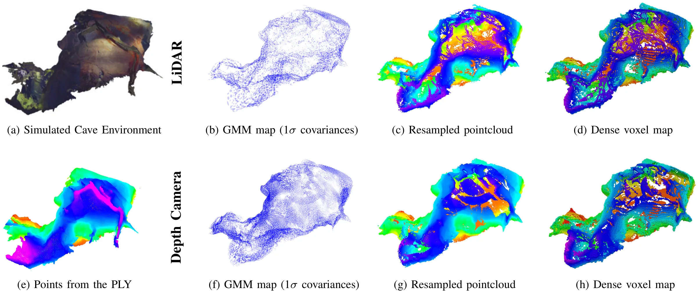
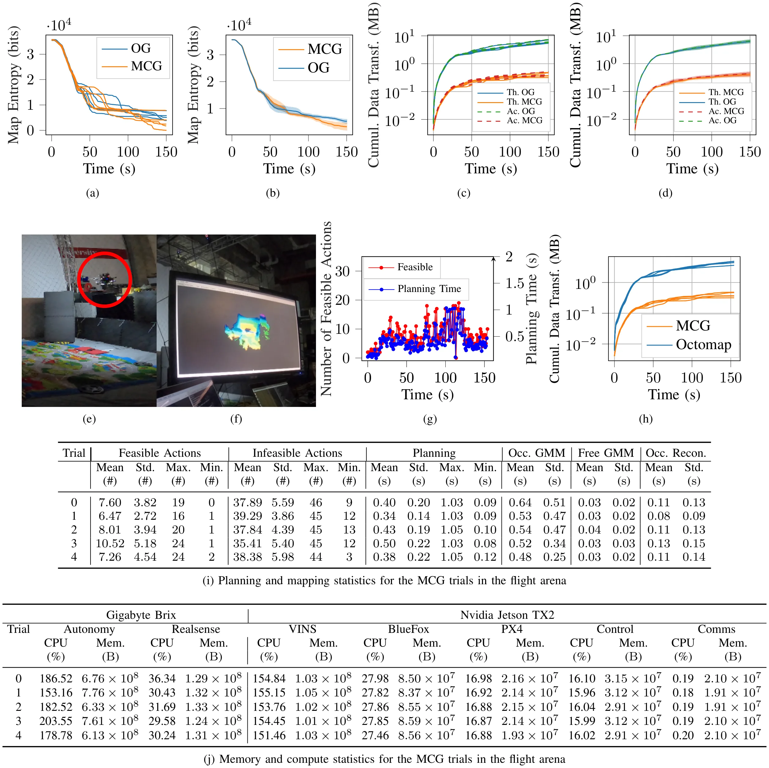
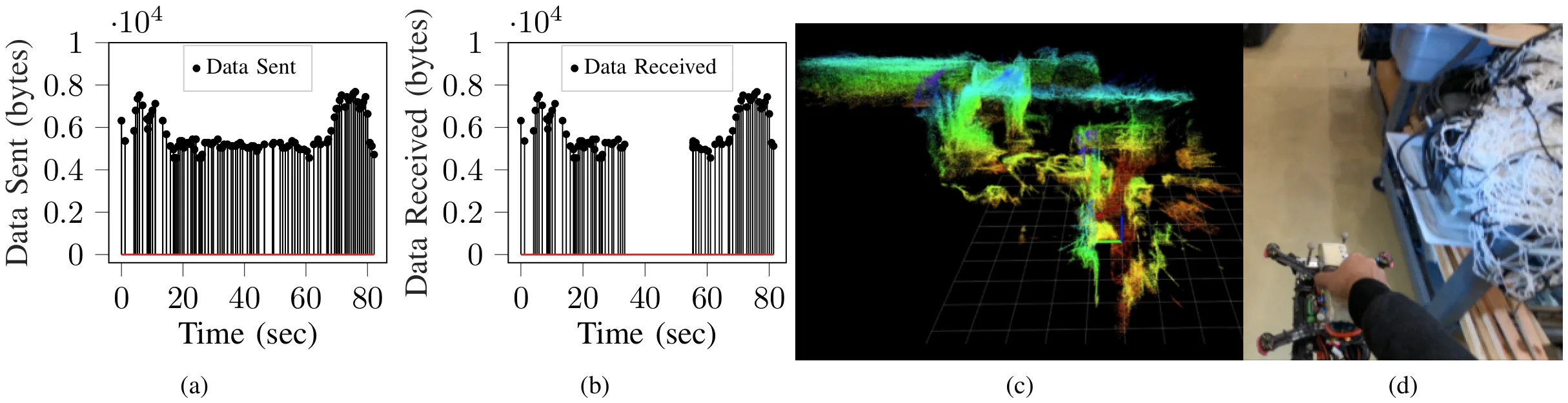
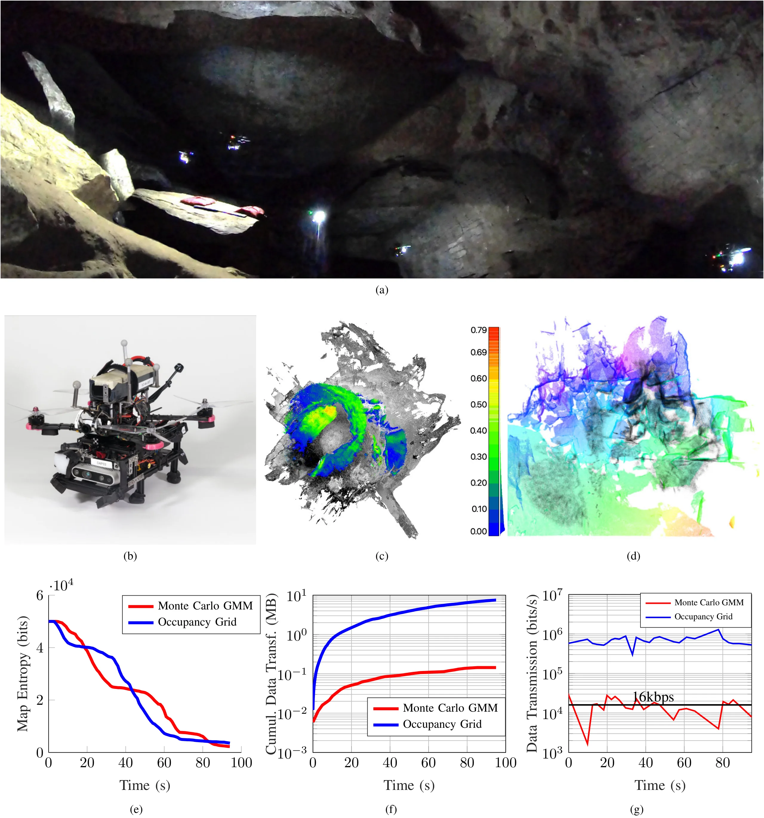
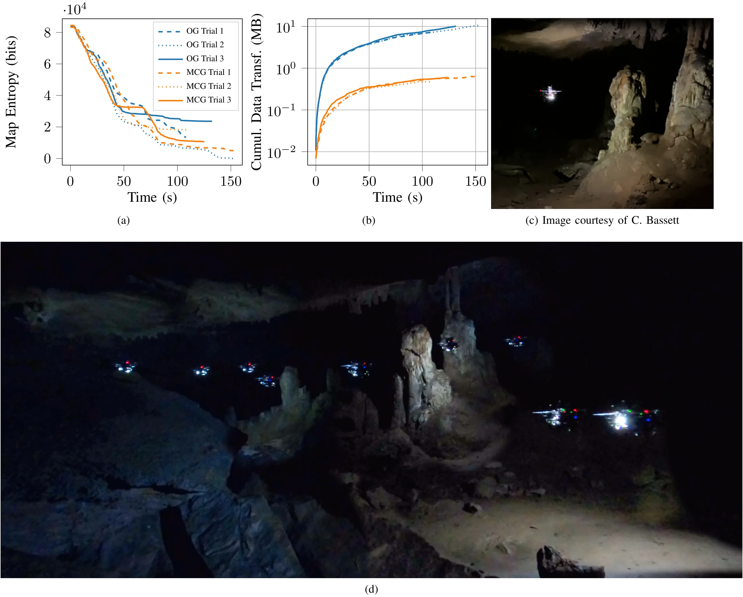
This paper presents a method for cave surveying in total darkness using an autonomous aerial vehicle equipped with a depth camera for mapping, downward-facing camera for state estimation, and forward and downward lights. Traditional methods of cave surveying are labor-intensive and dangerous due to the risk of hypothermia when collecting data over extended periods of time in cold and damp environments, the risk of injury when operating in darkness in rocky or muddy environments, and the potential structural instability of the subterranean environment. Although these dangers can be mitigated by deploying robots to map dangerous passages and voids, real-time feedback is often needed to operate robots safely and efficiently. Few state-of-the-art, high-resolution perceptual modeling techniques attempt to reduce their high bandwidth requirements to work well with low bandwidth communication channels. To bridge this gap in the state of the art, this work compactly represents sensor observations as Gaussian mixture models and maintains a local occupancy grid map for a motion planner that greedily maximizes an information-theoretic objective function. The approach accommodates both limited field of view depth cameras and larger field of view LiDAR sensors and is extensively evaluated in long duration simulations on an embedded PC. An aerial system is leveraged to demonstrate the repeatability of the approach in a flight arena as well as the effects of communication dropouts. Finally, the system is deployed in Laurel Caverns, a commercially owned and operated cave in southwestern Pennsylvania, USA, and a wild cave in West Virginia, USA.

Figures

**Field Deployment** Data and imagery excerpted from an exploration trial in a cave in West Virginia. (a) An autonomous aerial system explores and maps a formation. (b) A color image taken by the aerial system during exploration (the formation shown in (a) can be seen on the left-hand side of (b)). A depth image taken at the same time is shown in (c) and the resampled GMM map built during flight from the depth image is shown in (d). The video of the exploration trial corresponding to these images may be found at https://youtu.be/H8MdtJ5VhyU

**Cave Survey Map** An excerpt of the current working map for the cave on the Barbara Schomer Cave Preserve in Clarion County, PA. The map is encoded with terrain features. Note the passages marked too tight for human access in the top-right of the image. Aerial robots could be deployed to these areas to collect survey data. Image courtesy of B. Ashbrook.

**Manual Cave Sketching** A caver sketches a passageway to produce content for the map shown in Fig. 2. Image courtesy of H. Wodzenski. J. Jahn pictured.

**System Overview** Overview of the autonomous exploration system presented in this work. Using pose estimates from a visual-inertial navigation system (Section VI-C1) and depth camera observations, the mapping method (Section IV-A and Section IV-B) builds a memory-efficient approximate continuous belief representation of the environment while creating local occupancy grid maps in realtime. A motion primitives-based information-theoretic planner (Section V) uses this local occupancy map to generate snap-continuous forward-arc motion primitive trajectories that maximize the information gain over time.

**Sensor Observation Processing** Overview of the approach to transform a sensor observation into free and occupied GMMs. (a) A color image taken onboard the robot exploring Laurel Caverns. (b) A depth image corresponding to the same view as the color image with distance shown as a heatmap on the right hand side (in meters). (c) illustrates the point cloud representation of the depth image. (d) In the mapping approach, points at a distance smaller than a user-specified max range rd (in this case rd = 5 m) are considered to be occupied, and a GMM is learned using the approach detailed in Section IV-A1. Points at a distance further than rd are considered free, normalized to a unit vector, and projected to rd. The free space points are projected to image space and windowed using the technique detailed in Section IV-A2 to decrease computation time. Each window is shown in a different color. (e) The GMM representing the occupied-space points is shown in red and the GMM representing the free space points is shown in black. Sampling 2 × 105 points from the distribution yields the result shown in (f). The number of points to resample is selected for illustration purposes and to highlight that the resampling process yields a map reconstruction with an arbitrary number of points.

**Occupancy Reconstruction** Overview of the method by which occupancy is reconstructed. (a) The blue bounding box bt+1 is centered around Xt+1 and red bounding box bt is centered at Xt. (b) illustrates the novel bounding boxes in solid magenta, teal, and yellow colors that represent the set difference bt+1 \ bt. (c) Given a sensor origin shown as a triad, resampled pointcloud, and novel bounding box shown in yellow, each ray from an endpoint to the sensor origin is tested to determine if an intersection with the bounding box occurs. The endpoints of rays that intersect the bounding box are shown in red. (d) illustrates how the bounding box occupancy values are updated. Endpoints inside the yellow volume update cells with an occupied value. All other cells along the ray (shown in blue) are updated to be free.

**Limited FoV Approximation** For limited FoV sensors, the FoV is approximated by the illustrated blue and red rectangular pyramids. These FoVs may also be represented as tetrahedra. To determine if a sensor position should be stored, the overlapping volume between the two approximated sensor FoVs is found.

**Action Space Design** Action space design for the proposed information-theoretic planner. (a) shows a single motion primitive library generated using bounds on the linear velocity along {xB, zB} and the angular velocity along {zB}. (b) and (c) show top-down views of the motion primitive library collections used when the sensor model is a LiDAR [7] and a depth camera [36] respectively (off-plane primitives are not shown). The proposed planner can be used with either of these sensors using the appropriate action space designs explained in Section V-A.

**Simulation Statistics** Exploration statistics for simulation experiments. The first row of results pertains to the LiDAR sensor model and the second row to the depth camera sensor model. (a) and (d) illustrate the map entropy over time for 160 trials (80 trials per sensor model and 40 trials per mapping method), (b) and (e) illustrate the average map entropy over time for each method. Although both methods achieve similar entropy reduction, MCG uses significantly less memory according to the average cumulative data transferred shown in (c) and (f). When the LiDAR sensor model is used, the average cumulative data transferred at the end of 1500 s is 1.3 MB for the MCG approach and 256 MB for the OG approach. When the depth camera sensor model is used, the average cumulative data transferred at the end of 1500 s is 4.4 MB for the MCG approach and 153 MB for the OG approach. The MCG method represents a decrease of approximately one to two orders of magnitude as compared to the OG method for the LiDAR and depth camera sensor models, respectively. The experiments are conducted in the simulated cave environment shown in Fig. 9g. The four starting positions are shown as orange dots.

**Simulation Environment** The colorized mesh used in simulation experiments is shown in (a) and produced from FARO scans of a cave in West Virginia. After 1500 s of exploration with a LiDAR sensor model, the resulting (b) MCG map is shown with 1σ covariances and densely resampled with 1 × 106 points to obtain the reconstruction shown in (c). (d) illustrates the dense voxel map produced after a 1500 s trial with 20 cm voxels. (e) illustrates the pointcloud from the mesh shown in (a). (f) illustrates the MCG map with 1σ covariances, which is densely resampled with 1 × 106 points, to obtain the reconstruction shown in (g). (h) illustrates the dense voxel map with 20 cm voxels after 1500 s of exploration with the depth camera sensor model. The reconstruction accuracy for (c), (d), (g), and (h) are shown in Table II. All pointclouds shown are colored from red to purple according to z-height.

**Repeatability Trials** Results of repeatability trials for the MCG and OG approaches in a flight arena. (a) illustrates the entropy reduction for five trials for the MCG and OG methods. (b) plots the standard error on top of the mean line. The cumulative data transferred is provided for each approach in (c) with the mean and standard deviation for the trials shown in (d). The theoretical (Th. OG and Th. MCG) communications is compared to actual (Ac. OG and Ac. MCG) communications transmitted to the base station using UDP. (e) is a still image of the robot flying during one of the MCG trials (full video of the trial may be found at https://youtu.be/egwjv7YwHPE) and (f) illustrates the live map transmitted to the base station from the same trial. (g) provides a plot of the number of feasible actions in red with the planning time shown in blue. (h) Uses data from the MCG flights and generates an Octomap in postprocessing to compare the communications required. The Octomap performance is similar to that of the OG approach. More details about this analysis is provided in Section VI-C3. (i) and (j) provide timing, compute, and memory statistics for each subsystem for each of the five MCG flights. The figures reported in Fig. 11j are averages.

**Communication Dropout Test** Results of forcing a communication dropout on the system. The aerial system is carried through a research lab and down a hallway away from the base station and router to force a communications dropout. The accompanying video may be found at https://youtu.be/UVn2BbMQRJg. (a) illustrates the data sent from the robot and (b) is the data received by the base station (note: the base station and robot do not have their clocks synced). (c) illustrates the live map produced by the base station. (d) illustrates a view of the aerial system at the start of the experiment from a camera mounted on the operator's helmet.

**Laurel Caverns Exploration** (a) A single aerial system explores the Dining Room of Laurel Caverns in Southwestern Pennsylvania. Still images of the robot exploring the environment are super-imposed to produce this figure. (b) The aerial system with dimensions 0.25 m × 0.41 m × 0.37 m including propellers carries a forward-facing Intel Realsense D435 for mapping and downward-facing global shutter MV Bluefox2 camera (not shown). The pearl reflective markers are used for testing in a motion capture arena but are not used during field operations to obtain hardware results. Instead, a tightly-coupled visual-inertial odometry framework is used to estimate state during testing at Laurel Caverns. (c) illustrates the reconstruction error of the resampled GMM map as compared to the FARO map by calculating point-to-point distances. The distribution of distances is shown on the right-hand side. The mean error is 0.14 m with a standard deviation of 0.11 m. In particular, there is misalignment in the roof due to pose estimation drift. (d) A subset of the resampled GMM map (shown in black) is overlaid onto the FARO map (shown in colors ranging from red to purple) that displays the breakdown in the middle of the Dining Room. (e) The entropy reduction and (f) cumulative data transferred for one trial for each of the Monte Carlo GMM mapping and OG mapping approaches are shown. The communication is a theoretical calculation – not actual transmitted data. While the map entropy reduction for each approach is approximately similar, the GMM mapping approach transmits significantly less memory than the OG mapping approach (0.1 MB as compared to 7.5 MB). (g) illustrates the bit rate for each approach in a semi-logarithmic plot where the vertical axis is logarithmic. The black line illustrates how the approaches compare to 16kbps. For comparison, 16kbps is sufficient to transmit a low resolution (176 × 144 at 5 fps compressed to 3200 bit/frame) talking heads video [48, 49].

**West Virginia Cave Results** Overview of the results from experiments in a cave in West Virginia. (a) The map entropy over time for three trials of the MCG and OG approaches. (b) The data transferred between a robot and base station for each trial. The communication reported is actual transmitted data over UDP to a base station. Note that while the exploration performance is similar for both approaches, the data transferred for the MCG approach is substantially less. (c) A still image of the robot flying near a formation with terminated growth. (d) A composite image of one exploration trial composed of still images.

Acknowledgments

The authors thank C. Bassett for faciliating experiments at the West Virginia cave. The authors also thank H. Brooks and R. Maurer for facilitating experiments at Laurel Caverns and thank D. Cale for granting permission to test at Laurel Caverns. The authors also thank D. Melko for support and guidance regarding test sites, lending equipment and teaching the authors about caving. The authors thank B. Ashbrook for his insights and information regarding the cave on the Barbara Schomer Cave Preserve in Clarion County, PA. The authors thank H. Wodzenski and J. Jahn for providing images used in this work. Finally, the authors thank X. Yang for fruitful discussions about motion primitives-based planning and A. Dhawale, A. Desai, E. Cappo, T. Lee, M. Collins, and M. Corah for feedback on this manuscript.

BibTeX

@article{autonomous-cave-surveying-2022,
  title={Autonomous Cave Surveying with an Aerial Robot},
  author={Wennie Tabib, Kshitij Goel, John Yao, Curtis Boirum, and Nathan Michael},
  journal={IEEE Transactions on Robotics, Apr. 2022},
  year={2022}
}